Classifying Music Genres with a CNN

1 Introduction

The purpose of this project was to create a convolutional neural network that classifies the genre of music from audio files with a higher accuracy than the current baseline predictions. The baseline of predictions uses various classification models to find common patterns in the numerical measurement of audio features extracted from music files differentiated by genre. Classification using audio features produces good results, but researchers have proposed the idea of classifying the image representation of the audio file using a CNN to see if we can do even better. The model was then integrated into a simple and user-friendly web application for demonstration purposes. The dataset used in this project has over 100,000 songs in the form of MP3 files, and along with that comes a CSV file that contains the 518 engineered audio features that were extracted from each MP3 file. Theoretically, songs with similar features, or similar genres, should cluster together when plotted in a high dimensional vector space. These audio features work well with machine learning classification models, where the labeled output for this project is the genre of music associated with the .mp3 file.

1.1 Benchmark Analysis on Audio Features

This project begins with the exploration of genre classification using the extracted audio features methods. Various machine learning classification models were explored to get the highest prediction accuracy to serve as a benchmark for comparison with the CNN method. Applied models include Logistic Regression (LR), k- Nearest-Neighbors (kNN), Decision Tree (DT), Multilayer Perceptron Neural Network (MLP), and Linear, Polynomial, and Radial Basis Function Support Vector Machines (SVM). The highest prediction accuracy to serve as the benchmark was 63%, using an RBF kernel SVM and the following audio features: mel-frequency cepstrum coefficients (MFCC), contrast, and spectral centroid. The SVM works by finding the optimal hyperplane to separate the data in two dimensions if the data is not linearly separable. Using the audio features, the SVM parameters can be tweaked through trial and error to discover an optimal margin of the hyperplanes that separate the data. For now, that optimal margin was found using an RBF kernel and default gamma, 𝛾.

1.2 Featureless Analysis with a CNN

Convolutional neural networks, like ordinary neural networks, consist of neurons that have learnable weights and biases. The network computes a loss function on the last fully connected layer and updates its neurons during the backpropagation process. CNNs differ in that they are altered to handle inputs in the form of images, rather than tables of labeled features. Thus, in order to use a CNN for genre classification, one must input genre labeled images that represent the audio files instead of a table of labeled audio features, which begs the question: How do you visually represent an audio file?

2 Audio Signal Processing

The process of creating a visual representation from audio files to serve as input into a CNN follows a series of transformations of signal data. The user typically has .mp3 files in their music library, which is an audio file, not an image, but we can transform these files into images for classification purposes. This project uses the Librosa Python package and its many functionalities to make a series of file conversions in the following order:

1. Moving Picture Experts Group (MPEG) Audio Layer-3 (.mp3)
2. Waveform Audio File Format (.wav)
3. Waveform Image: Amplitude vs. Time (.png)
4. Periodogram: Magnitude vs. Frequency (.png)
5. Spectrogram: Frequency vs. Time (.png)
6. Mel Spectrogram: Mel Scale Frequency vs. Time (.png)

This process begins by converting an .mp3 file to a .wav file. The Waveform Audio File Format (.wav) is an audio file format standard, developed by IBM and Microsoft, for storing an audio bitstream on PCs. The bitstream is a series of 0s and 1s that represent the signal of the audio. A signal is a of variation in air pressure measured by taking samples of the air pressure over a period of time. The rate at which the air pressure is sampled is called the sample rate, and a common sample rate is 44.1kHz, or 44,100 samples per second. This signal data is plotted to create a waveform, which is an image.

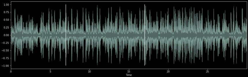
Great! We have an image. Why not pass this through the CNN? Well right now, the waveform is relatively visually similar to other waveforms of completely different genres. Thus, much like a human, the CNN will have a difficult time distinguishing patterns for different genres between waveforms, so we seek to transform this data into something more useful, and we can do so using the Fourier transformation.

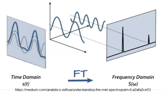
An audio signal consists of many single-frequency sound waves. When taking samples of the signal over time, we only capture the resulting amplitudes. The Fourier transformation is a mathematical formula that decomposes a signal into its individual frequencies and the frequency’s amplitude. Thus, it converts the signal from the time domain into the frequency domain, which is called a spectrum. The way this works is through decomposing the signal into a set of sine and cosine waves that add up to the original signal.

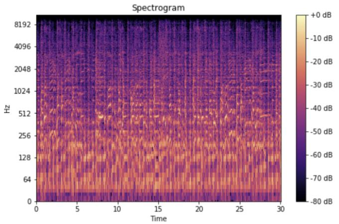
The fast Fourier transform (FFT) is an algorithm that allows us to analyze the frequency of a signal, which is great, but the frequency of our music signals vary over time. Thus, we need a way to represent a non-periodic spectrum of these signals as they vary over time. To achieve this, the FFT is computed on overlapping windowed segments of the signal to produce a spectrogram. Thus, a spectrogram is essentially a bunch of FFTs stacked on each other, and it visually represents a signal’s loudness, or amplitude, as it varies over time at different frequencies. The y-axis is converted to a log scale, and the color dimension is converted to decibels, which is also on a log scale because humans can only perceive a very small and concentrated range of frequencies and amplitudes.

Studies have shown that humans do not perceive frequencies on a linear scale. We are better at detecting differences in lower frequencies than higher frequencies. Thus, in 1937, researchers proposed a unit of pitch such that equal distances in pitch sounded equally distant to the listener, measured on what is now called the mel scale. The Mel Spectrogram is simply the spectrogram with frequencies converted to the mel scale, and all these transformations were made possible using the Librosa Python package. Now we’re ready to pass this through our CNN, but first a little context on why we’re using a CNN.

3 Related Work

In 2017, a team of researchers introduced the dataset, titled “FMA: A Dataset for Music Analysis”. FMA stands for Free Music Archive, so all the music provided in the dataset is copyright free. There are plenty of other music archives, some much larger than this one, but this data is unique in that it includes the engineered audio features for each song. This was necessary to save time from having to create audio features for songs in another large dataset using Librosa.

The authors of this paper have already completed benchmark analyses using various machine learning models that consider the audio features, but the accuracies of the genre classification did not exceed 63% using their own medium sized dataset, with the best results coming from a support vector machine model. They ended their paper with the proposal that someone could try to improve on this using neural networks that analyze only the waveform.

About a year later, another team released their work where they proposed a Convolutional Neural Network to identify an artist from an audio’s spectrogram. After training their Convolutional Neural Network model, they fed it songs with the intention to find Similar songs, and they did so with about 72% test accuracy, which means that their CNN was successful in distinguishing patterns of significance in the spectrograms between genres. Thus, from here it would be interesting to play around with the various layers in a CNN model to get that prediction accuracy even higher.

4 Results

4.1 Benchmark Results

Of the 518 features, some are more useful than others, and perhaps some of them cause more noise and overfitting than they are helpful. Through trial and error, using only the MFCC, contrast, and spectral centroid features produced the best prediction accuracies, with MFCC being the most important. MFCC is a set of coefficients that describe the shape of spectral envelope. Contrast measures the difference between foreground noise, such as speech, and background noise, such as instrumentals. Spectral Centroid characterizes where the center of mass of the spectrum is located.

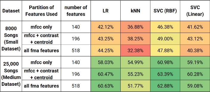
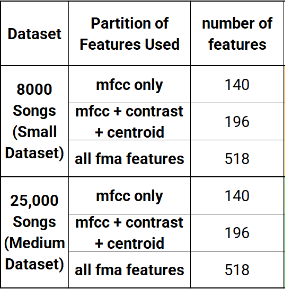
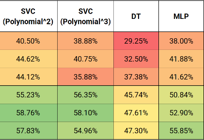
Unsurprisingly, results from the larger “medium dataset” provided higher prediction accuracies. The results from this project matched the results from the FMA research paper with a maximum of 63% prediction accuracy using an SVM.

Understanding how this process works helped rationalize why a different approach might be appealing. The process of extracting audio features for a large dataset of audio files is a time-consuming process, but of course, this only needs to be done each time we train our model. Thus, if it produces better results then why not. Fortunately, better results were found using the CNN method.

4.2 CNN Results

For this model, the data was rearranged into 9 genre folders, each with 1000 audio files, which is comparable in size to the organization of the small dataset of audio features. The audio files were shuffled and then train - test split 90 – 10.

The CNN model is built using Keras, consists of 6 convolutional layers, a dropout layer to reduce over-fitting, and a dense layer with a SoftMax activation to output genre probabilities. The model is trained for 100 epochs, with a learning rate of 𝛼 = 0.00005, a 30% dropout rate, a 3 x 3 kernel size, and 6 convolutional layers, which resulted in a training accuracy of 99.7%, a test/validation accuracy of 83%.

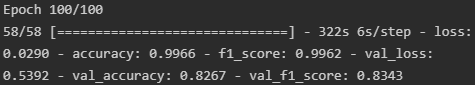
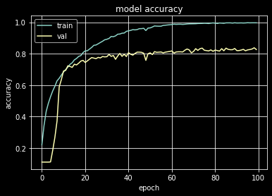
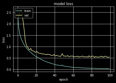
The training accuracy is much higher than the test accuracy, which may be due to the dataset being on the smaller side. I think that the model is probably capturing the patterns inside the training data and overfits a bit because the variance of the larger training set is greater than the smaller test set.

5 Web Application and Analysis of Classifications

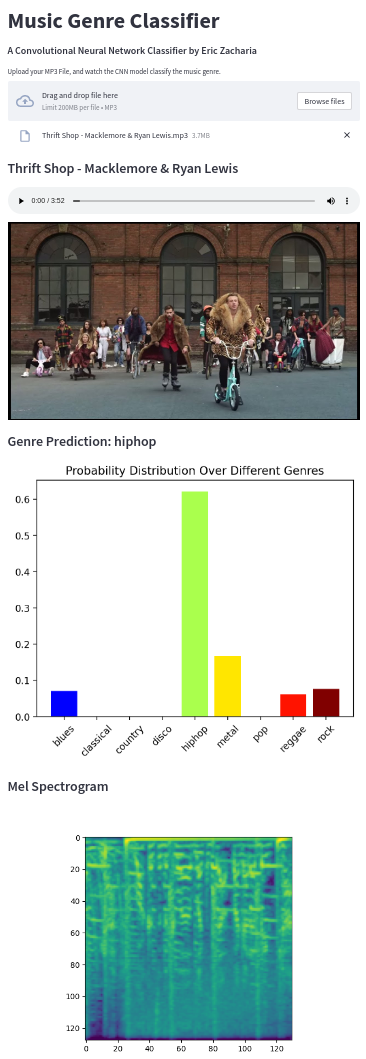
The application of this model was created to demonstrate the success of the CNN model’s prediction capabilities on songs of the user’s choosing.

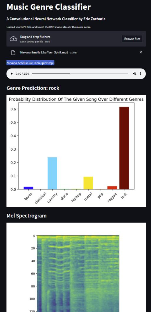
First, the user is prompted to either browse or drag- and-drop an .mp3 file to be uploaded for genre classification. The background pipeline then processes this .mp3 file by making its transformations from waveforms to mel spectrograms to be assessed by the pretrained CNN model. The application makes its prediction, and outputs the SoftMax probabilities for all genres under consideration, as well as the mel spectrogram image representing the song of choice.

The web application was built using the Streamlit Python package, which handles the web formatting, so the application looks nice without much effort. Below is a screenshot of the application after uploading the rock song, “Smells Like Teen Spirit”.

After testing various songs from my personal music library, I would concur that approximately 4 out of 5 songs are classified correctly, but some genres have better performance than others.

Often the songs that were misclassified were arguably in a gray are between genres. One particularly interesting example of an incorrect classification was found with the rock song “Learn to Fly” by the Foo Fighters, which the model classified as metal, but many others would classify it as rock.

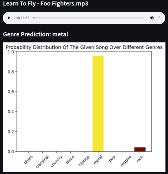
For those who are not familiar, The Foo Fighters is a rock band, but their lead singer generally has a loud style of singing, which is a common theme found in metal music. Thus, I don’t find this misclassification to be surprising, but I do think that customers using a music service like this would have an issue with such a mistake.

5.1 Thinking Like a Machine

I decided to investigate why such misclassifications might be happening with hope that I could unveil the problem for a future solution.

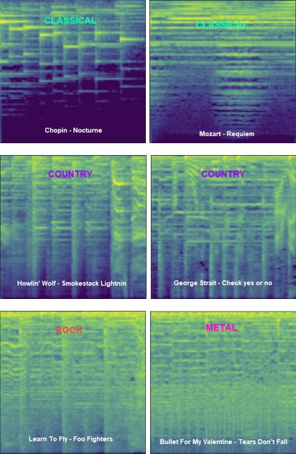
Thinking like a machine, the convolutional neural network scans the pixels in the image for common patterns found in contrasting pixel edges. Basically, I figured that if I can personally distinguish between photos of cats and dogs, then perhaps I may be able to recognize differences between genres in the Mel Spectrograms that are being fed into the CNN.

As you can see in the following figures, there are distinct differences between genres of music. While the two Spectrograms from each Genre Example do not look exactly alike, you might be able to imagine how the model is generalizing these patterns as similar. The bottom row displays the spectrograms for two songs classified as Metal, but “Learn to Fly” is more popularly known as Rock. So clearly, there exists some gray area between genres, but the rock song’s spectrogram does look strikingly similar to the spectrogram of the metal song, compared to the other genres in the figure.

This presents a challenge to the model to correctly classify songs that reside in gray areas between genres, but genre classification is somewhat subjective anyways, right? I find it helpful to imagine this classification as the machine’s unbiased opinion based solely on the spectrogram image it studies. It is not told by anyone that most people would classify this song as rock, or that the song comes from a rock band. It makes up its decision without any biases based on signal data, and this can only get better with more training and tweaking.

6 Areas of Improvement

While the prediction accuracies appear to be very high, I have been able to identify some of its struggles through experimentation with audio files.

The model to have an issue with misclassifying songs that are relatively louder than others as metal songs, and I think this can be avoided. With some tweaking to the CNN parameters, the overall accuracy can be improved, and with more music, some gray-area music genres can be classified better. For example, there is a significant difference in the spectrograms between old country songs and new country songs. New country appears more so like rock and pop, while the model is trained more so on old country. This can be improved upon with more genre classes for prediction and with more data that encompasses more sub-styles within each genre.

This of course can be helped with adding more data, which is certainly available, and possible to implement with more time to work on this project.

Also, besides just throwing more data at the model to train on - I think the overfitting issue can be mitigated with some cross validation on the data so it can find a more optimal splitting of training and testing data.

7 Effort

Initially I did a lot of research on SVMs because I wanted to see if I could beat the FMA research paper’s benchmark prediction accuracy using the extracted audio features. I ended up matching their accuracy using the same size dataset and chose to move on for the sake of time.

The decision to work with audio data instead of image data or only tabulated feature data presented a lot of room for learning about audio signal processing and refamiliarizing myself with convolutional neural networks.

I did some deeper research into CNNs, which have a lot of options for fine tuning the model available, such as picking an optimal learning rate, kernel size, stride, dropout rate, and number of layers. Playing around with these parameters ultimately improved the performance of my model.

Learning everything audio signal processing was probably the most complex task. I began with studying the terminology found in the extracted feature data so I could understand what I was working with, which helped me discover which features might have more importance than others, and which might be noise in the model. Next, understanding the transformation process from .mp3 files to mel spectrograms was pertinent to the success of the CNN model. This model’s higher prediction accuracy would not be possible without the mel spectrogram, and all these transformations would not have been doable within the timeframe of this project without the Librosa library. Thus, learning the methods available in Librosa to make these transformations possible was necessary, given the time available to work on this project.

Already having learned PyTorch in the past, I chose to expose myself to TensorFlow and Keras, for resume building purposes. They are extremely similar, and the documentation helped me realize the similarities.

I learned about streamlit from friends in the Data Science community. It is a popular Python package amongst data scientists who want to get their models into nice looking web applications with minimal effort, and it is well documented – making it easy for me to quickly get my own web application running.

8 Conclusion

I would be very interested to know if models like this one are currently used at large companies for similar purposes. I wonder how they might handle mistakes in classification, such as initially publishing results like “Learn to Fly is metal” and later correcting those mistakes that come to light from their customer base. Or perhaps their models have much higher prediction accuracies, and this problem is not so prevalent.

After running through both methods, I believe that the CNN has a lot more potential for success compared to the method of extracting audio features. Better results were found using less data. One advantage to the audio features is not needing to keep the audio files after extracting the features, so if computer memory is an issue, then perhaps one might be interested in pursuing the optimization of audio feature models.

Web Application

References

1. Michaël Defferrard, Kirell Benzi, Pierre Vandergheynst, Xavier Bressony, 2017. "FMA: A Dataset for Music Analysis"
2. Librosa – Audio and Music processing in Python Library
3. Leland Roberts. 2020. "Understanding the Mel Spectrogram"
4. Jiyoung Park, Jongpil Lee, Jangyeon Park, Jung-Woo Ha, Juhan Nam. 2018. "Representation Learning of Music Using Artist Labels"
5. Keras deep learning API Python Library.
6. Streamlit – easy web apps for data science Python Library.
7. Scikit-learn SVM Classifier.
8. Benjamin Murauer, Günther Specht. 2018. "Detecting Music Genre Using Extreme Gradient Boosting"
9. Seth Adams. 2018. “DSP Background – Deep Learning for Audio Classification (p.1 & p.2)”

Appendix

A.1 Benchmark Results

The source code for this project with instructions on how to run the web application can be found in my GitHub repository.

A.2 Video Presentation

The video presentation for this article can be found here on YouTube.

A.3 Journal Article

PredictingTheGenreOfMusicWithCNNs.pdf